(This blog post is our joint effort with Sergei, all typos and missing Oxford commas are mine). The quest to make massively parallel computation easily accessible to everyone has been a daunting one for many generations of computer scientists and engineers. While far from being complete, with cloud computing infrastructure available through Amazon EC2, Google Compute Engine, and other similar platforms a significant milestone has been reached. At the same time the quest to establish rigorous theoretical foundations of massively parallel computing has led to development of multiple theoretical models. Despite different modeling assumptions underlying these models, many parallel algorithmic techniques can be used in some or all of them with minor modifications. Moreover, in some restricted scenarios even direct simulations are available. In this post we discuss some of the most popular theoretical models for parallel computing and the relationships between them.

MapReduce

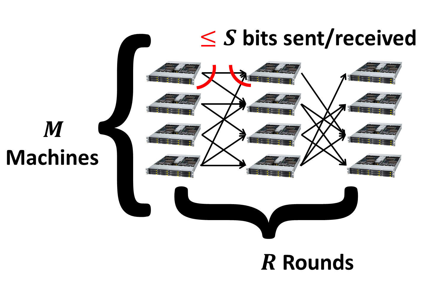
We will strongly emphasize connections between these different models and the modern MapReduce model for computation in the cloud (MRC) that we described here. As a reminder, the MRC model is specified by the number M of identical machines each having S local memory.

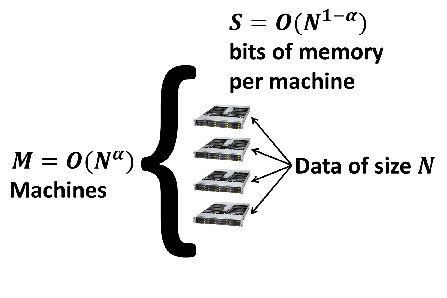
The goal of the algorithm design is to minimize the number of parallel rounds of computation which we denote as R. In each communication round the number of bits sent and received by each machine is at most S (in fact, in most cases only the bound on the incoming communication matters).

We will use the Minimum Spanning Tree (MST) problem as a benchmark for comparison between the models. In MRC the MST problem can be solved in constant number of rounds for sufficiently dense graphs. As shown through a filtering technique by Lattanzi et al. here for graphs with \(|E| = n^{1 + c}\) edges \(\lceil c/\epsilon\rceil\) rounds suffice assuming \(M = O(n^{1+\epsilon})\) and \(S = O(n^{c-\epsilon})\) so that the total space is \(M * S = O(|E|)\).

Bulk Synchronous Parallelism

The Bulk Synchronous Parallel model (BSP) was introduced by Leslie Valiant in 1990 in his seminal article “A Bridging Model for Parallel Computation”. While this model has been subsequently refined to capture multicore computing in 2008, here we focus on the original BSP model. BSP and MRC are very closely related. The key idea behind BSP is breaking computation into synchronized supersteps and it later formed the basis in MRC.

BSP computation assumes a set p of processors, each with local memory. Moreover, the computation proceeds in a series of global synchronized supersteps. There are three parameters that are combined to give the cost of a BSP computation:

• The number of processors, p.
• The number of timesteps needed to synchronize, l (communication latency).
• The number of timesteps needed to send one word of memory to a different machine, g (communication gap).

Some of the descriptions of the models also include the speed of each processor (instructions/sec), s. But we can easily factor that out when working with homogeneous machines.

The cost of a superstep where each processor does at most x operations and sends/receives at most h words is then: l + x + g * h.

The total work is p times the cost of the superstep, and the efficiency is the ratio of the best sequential algorithm to the total work (over all supersteps). Note that since latency and gap may depend on the number of processors, the total cost is superlinear in the number of processors.

One of the goals of BSP was to give the analytically best algorithm for different settings of the parameters. This would allow one to decide what is the fastest or most work efficient algorithm for a particular setting. It is not surprising then that some of the early work focused on how to minimize values of g, l in various network topologies (torus, hypercube, butterfly, etc.). Additional work also measured these across different networks realized in practice.

One way to generalize the BSP model is to model the fact that communication costs are not linear (sending 1Mb between machines is much cheaper than sending 1,000,000 distinct one byte messages.) We can model this by letting G() be a function of the number of words sent. In traditional BSP then, \(G(h) = g * h\). In the MRC model of computation, \(G(h)\) is discretized – with \(G(h) = \lceil h / S\rceil * K\) for some large constant K that dwarfs all computation costs. Such choice of a cost function implies that in order to best use communication the computation should be broken into rounds with at most \(S\) bits sent between the rounds. In MRC l is taken to be O(1) as synchronization can proceed at any time.

Due to a large number of parameters the algorithmic results in the BSP model tend to be bulky to state. We refer the reader to this paper by Adler et al. for the details of the MST algorithm in the BSP. To the best of our knowledge there aren’t many algorithmic results in the BSP model. This might be partially due to its invention having been ahead of its time and partially due to a large number of parameters which makes it not very friendly for algorithm design. One of the key contributions of the MRC model is reduction in the number of parameters making algorithmic results cleaner and easier to state and compare.

Parallel Random Access Machines

The model is characterized by:

• The number of processors, p.
• The size of the shared memory, m.
• The size of local memory available to each processor, l.

Furthermore, read/write access to the shared memory might be implemented differently:

• ER/CR: Exclusive Read/Concurrent Read allow to perform read access to each shared memory cell either to only one processor (ER) or to any number of processors (CR) during each superstep.
• EW/CW: Exclusive Write/Concurrent Write allow to perform write access to each shared memory cell either to only one processor (EW) or to any number of processors (CW). In case if multiple write operations occur to a shared memory cell under CW there exist multiple policies for resolving which value is going to be written (priority-based, random, arbitrary, etc.).

Among four possible combinations of read/write access rules only three are typically considered: EREW, CREW, and CRCW (requires a specification of the conflict resolution policy). Since we only discuss PRAMs very briefly here, we refer the reader to this paper by Guy Blelloch and Bruce Maggs and this class at CMU for a comprehensive introduction to PRAMs.

A restricted class of EREW PRAM algorithms can be simulated in MRC with only a constant overhead in the number of rounds. The basic idea is the following. Assuming that:

• m + p * l < M * S (the total memory used by PRAM algorithm is less than the total memory available to MRC)
• l < S (local memory in PRAM is less than in MRC, which is reasonable given that typically p is much bigger than M)

one can simulate EREW access to all the \(m\) shared memory cells in \(O(1)\) rounds while using \(p * l\) memory to perform the local computations. This is done by assigning \((p * l) / S\) machines to simulate \(S/l\) PRAM processors each and \(m/S\) machines to simulate the shared memory cells. Since the read/write requests are exclusive they can be directly communicated between the simulated processors and the simulated memory cells. Note that simulating concurrent reads might overload the machines simulating the memory if much more than \(S\) requests are simultaneously submitted. See Theorem 7.1 here for the details (modulo the ER vs. CR issue discussed above). Also note that while the number of rounds is preserved well this simulation might lead to time-inefficient algorithms since multiple PRAM processors might be simulated sequentially on a single MRC machine.

Models with Restricted Communication

In models with restricted communication the input graph corresponds to a communication network between \(n\) machines. Initially each machine has the list of its neighbors as the input. Moreover, the communication is restricted in one of the two ways:

• Messages can only be sent over an underlying network between the machines, i.e. in every round each machine can only talk to its neighbors. In this case for graph problems which depend on the entire input the diameter of the network D often gives a lower bound on the number of rounds since messages must be propagated through the network.
• Messages are restricted in size. When discussing size-restricted messages below we will always assume that the bound on the message size is W = O(log n) where n is the input size.

The three models discussed below (LOCAL, CONGEST and CONGESTED CLIQUE) correspond to the three possible combinations of these two restrictions. In all these models the computational power of the machines is either unbounded or limited to polynomial time computation on their input. We discuss these models only briefly here since they are more applicable to settings such as sensor networks rather than massively parallel computing. A good introduction into algorithmic techniques is given in this class at MIT.

LOCAL

The most basic of the restricted communication models is LOCAL. In this model the communication is restricted to the underlying network while message size is unbounded. This allows to solve any problem trivially in D rounds. Lower bounds in this model show that \(\Omega(D)\) rounds are necessary for computing a Minimum Spanning Tree and 2-coloring even for instances as simple as an even cycle.

CONGEST

In the CONGEST model restrictions are imposed both on the communication network and the message size (W=O(log n)). Two flavors of these models exist: one that allows to send arbitrary messages and one that only allows each machine to broadcast the same message to its neighbors. Below we discuss the first of these two versions which has been studied more extensively. In this model the number of rounds necessary and sufficient for computing a Minimum Spanning Tree is \(\tilde O(D + \sqrt{n})\).

CONGESTED CLIQUE

Finally in the CONGESTED CLIQUE model we only have the message size restriction (W=O(log n)). In this model a Minimum Spanning Tree can be computed deterministically in \(O(\log \log n)\) rounds (Lotker, Patt-Shamir, Pavlov, Peleg ‘05). A recent preprint shows an \(O(\log \log \log n)\)-round randomized algorithm. This model is the closest of the three to the MRC model because there is no restriction on the communication topology. In some restricted scenarios there exist simulations of algorithms for CONGESTED CLIQUE in the MRC model, see here. However, in general the CONGESTED CLIQUE model is incomparable to MRC since both the outgoing and incoming communication for each machine are allowed to be linear in the input size while for MRC both are strictly sublinear. In particular, sparse graph connectivity can be solved in CONGESTED CLIQUE in one round by sending all edges to a single machine.

The “Big Data” Model

The “Big Data” model introduced in this paper is a generalization of the CONGESTED CLIQUE model. Instead of having the number of machines being the same as the number of vertices in the graph, the number of machines is treated as a parameter \(k \le n\). The input graph is vertex partitioned between these \(k\) machines. In one round any pair of machines is allowed to communicate using messages of size W=O(log n). Close relationship to the CONGESTED CLIQUE model allows to reuse existing algorithmic techniques. Near-optimal results for many fundamental problems in the “big data” model are given here. In particular for computing a Minimum Spanning Tree \(\tilde O(n/k)\) rounds are necessary and sufficient.

Among all models with restricted communication the “big data” model is the one most similar to MRC. However, a hard bound on communication leads to very strong lower bounds in this model such as the \(\tilde \Omega(n/k)\) lower bound for MST discussed above.

---