In this post I will introduce a theoretical model for computation in centralized distributed massively parallel computational systems (or in short clusters like those used by Google many other companies). Over the last decades the supercomputer architecture has moved towards such designs and there seem to be no signs of this trend slowing (see Wikipedia article for more information).

MapReduce-style Computation
MapReduce is a programming model for cluster computing introduced by Jeff Dean and Sanjay Ghemawat in their seminal paper. There exist multiple different implementations of MapReduce, Apache Hadoop being one of the most popular among them.

Below I will describe a theoretical version of the model for MapReduce-style computation. This model is easy to understand, avoiding low-level technical details involved in the implementation of the MapReduce model. For those familiar with the standard MapReduce implementations, which use key-value pairs and Map/Shuffle/Reduce phases, let me just say that these two are interchangeable abstractions of the same thing.
This model has emerged in a sequence of papers:
- Jon Feldman, S. Muthukrishnan, Anastasios Sidiropoulos, Clifford Stein, Zoya Svitkina: On distributing symmetric streaming computations. SODA 2008.
- Howard J. Karloff, Siddharth Suri, Sergei Vassilvitskii: A Model of Computation for MapReduce. SODA 2010.
- Michael T. Goodrich, Nodari Sitchinava, Qin Zhang: Sorting, Searching, and Simulation in the MapReduce Framework. ISAAC 2011
- Paul Beame, Paraschos Koutris, Dan Suciu: Communication steps for parallel query processing. PODS 2013
Storage Model
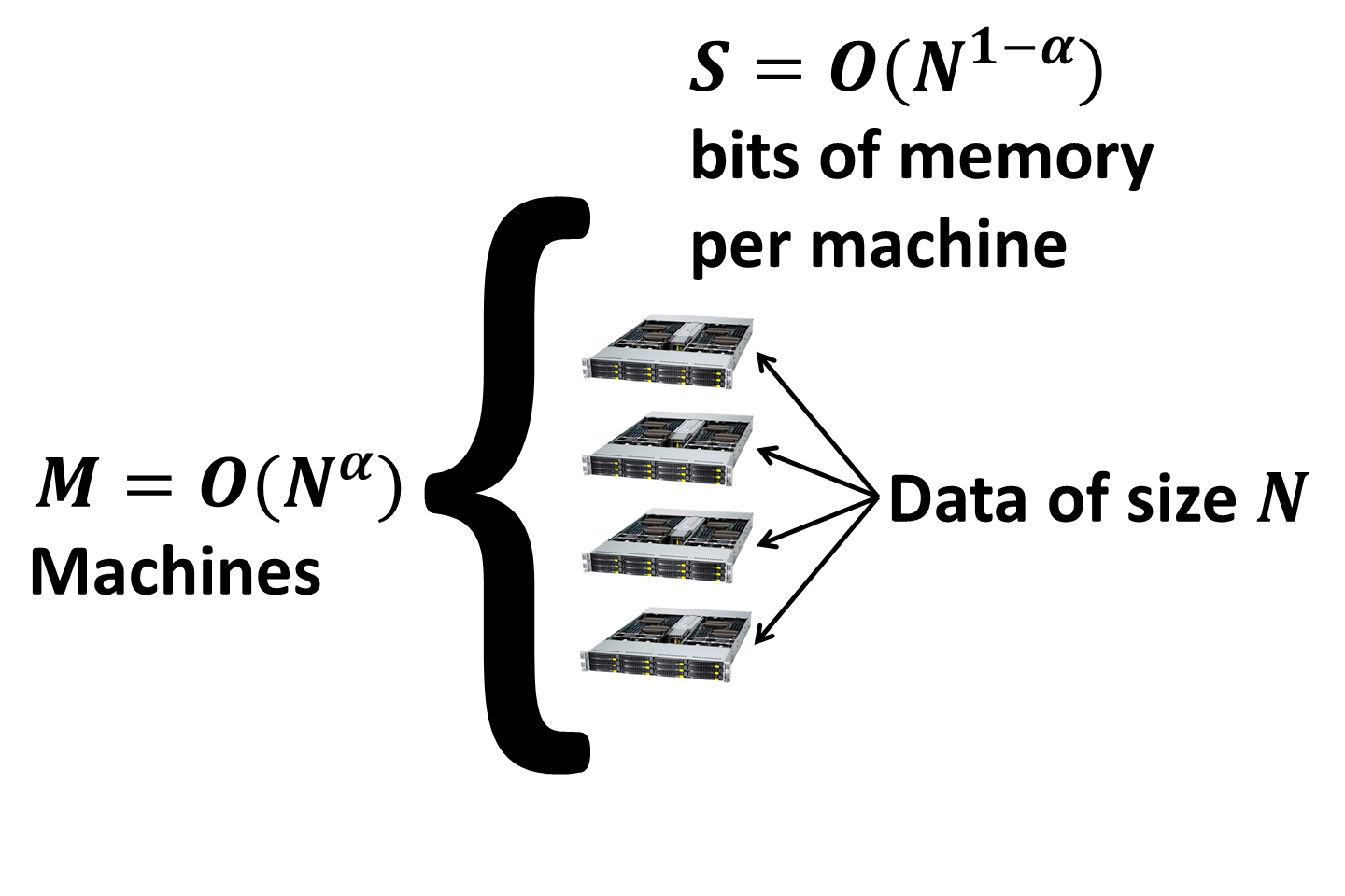
First, let’s discuss the data storage. Data of size \(N\) is partitioned between \(M\) identical machines. Each machine is the standard RAM machine with \(S\) bits of RAM. The data fits into the overall memory with possibly some extra memory left for the algorithm to use so that \(M \times S = C \times N\), where \(C\) is an overhead replication factor. Unless otherwise specified, replication will be constant, i.e. \(C = O(1)\) so I will ignore it.
Without loss of generality I will assume that \(M = O(N^\alpha)\) and \(S = O(N^{1 - \alpha})\). Here \(\alpha\) is a constant, which is typically significantly greater than zero, but less than \(1/2\) (think of a cluster with thousands of machines, each having gigabytes of RAM).
Computational Steps
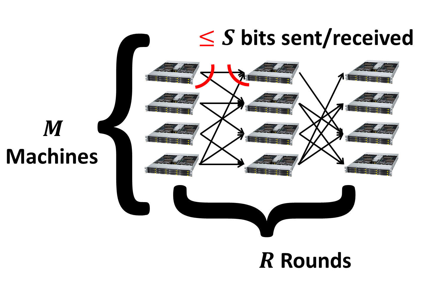
The key parameter in the study of massively parallel algorithms is the number of supersteps (or rounds) of computation. The entire computation is divided into such rounds, each consisting of two phases:
-
Local computation phase. In this phase each machine performs a local computation based on its data. This computation should be as efficient as possible (ideally linear or close to linear time, sometimes allowing polynomial time for particularly hard problems). Typically local running times for all machines will be identical at a given round so let’s denote them as \(T_i(S)\) at round \(i\).
-
Communication phase. In the communication phase each machine can send and receive at most \(S\) bits of information. The limitation on received data comes from the memory bound of every machine. Note that this doesn’t allow, say, streaming computations to be performed on the fly on the incoming data. The limitation on sent data comes from the technical details of the MapReduce framework. For those familiar with the low-level details I will just say that the key-value pairs have to be stored locally before they get redistributed between machines.
Number of Rounds
Overall, if the number of rounds is \(R\) then the total local computational time is \(\sum_{i = 1}^R T_i(S)\). The total communication time is \(R \times CC(N)\), where \(CC(N)\) is the time it takes to redistribute the data between machines in each round. This parameter is dependent on the under the hood implementation of the system so I will assume it as given.
For example, if local running times are linear then we get total running time of \(R \times (O(S)+ CC(N))\). This emphasizes the number of rounds \(R\) as the key parameter for understanding the complexity of algorithms in MapReduce-like systems. Other considertaions, such as fault-tolerance, also suggest that ideally we would like to have just a few rounds. So having \(O(1)\) rounds is great, while \(O(\log N)\) rounds might be also ok for some problems.

Examples
Let’s look at some examples of how many rounds it takes to solve some basic problems:
- Sorting. \(O(\log_S N) = O(1)\) rounds suffice to sort \(N\) numbers. This is a result from: Michael T. Goodrich, Nodari Sitchinava, Qin Zhang: Sorting, Searching, and Simulation in the MapReduce Framework. ISAAC 2011.
- Connectivity. \(O(\log N)\) rounds suffice to check whether a graph with \(N\) edges is connected or not. This is a result from: Howard J. Karloff, Siddharth Suri, Sergei Vassilvitskii: A Model of Computation for MapReduce. SODA 2010.
In practice it takes two rounds for a terabyte dataset using TeraSort, which uses essentially the same algorithm as the theoretical \(O(\log_S N)\)-round algorithm mentioned above. Here is a simplified version:
- Take a random sample of size \(M - 1\).
- Assuming that \(M \le S\) in the first round we can sort this sample locally on one of the machines, obtaining a sequence \(a_1 \le a_2 \le \dots \le a_{M-1}\).
- In the second round send all keys in the range \([a_{i - 1}, a_i)\) to the \(i\)-th machine and sort them locally on that machine.
The connectivity algorithm is more complex so I will describe it in more detail below.
Connectivity in \(O(\log N)\) rounds
The data consists of \(N\) edges of an undirected graph on the vertex set \(V\). The goal is to compute the connected components of this graph. For every vertex \(v \in V\) let \(\pi(v)\) be its unique integer id (a number between \(1\) and \(|V|\)). During the algorithm we will also maintain a label \(\ell(v)\) for each vertex \(v\). Let \(L_v \subseteq V\) be the set of vertices with the label \(\ell(v)\). During the execution of the algorithm this set will be a subset of the connected component containing \(v\). We will use \(\Gamma(v)\) and \(\Gamma(S)\) to denote the set of neighbors of a vertex \(v\) and a subset of vertices \(S \subseteq V\) respectively.
Here is a high-level description of the algorithm. I will call some of the vertices active. The idea is that every set \(L_v\) of vertices with the same label according to \(\ell\) will have exactly one active vertex during the execution of the algorithm.
- Mark every vertex \(v \in V\) as active and label \(\ell(v) = v\).
- For phases \(i = 1, 2, \dots, O(\log N)\) do:
- Call each active vertex a leader with probability \(1/2\). If \(v\) is a leader, mark all vertices in \(L_v\) as leaders.
- For every active non-leader vertex \(w\), find the smallest leader (with respect to \(\pi\)) vertex \(w^{\star} \in \Gamma(L_w)\).
- If \(w^{\star}\) is not empty, mark \(w\) passive and relabel each vertex with label \(w\) by \(w^{\star}\).
- Output the set of connected components, where vertices having the same label according to \(\ell\) are in the same component.
It is easy to see if for two vertices \(u\) and \(v\) it holds that \(\ell(u) = \ell(v)\) then \(u\) and \(v\) are in the same connected component. It remains to show that every connected component will have a unique label with high probability after \(O(\log N)\) phases. We will show that for every connected component in the graph the number of active vertices in this component reduces by a constant factor in every phase. Indeed, half of the active vertices in every component is declared as non-leaders. Fix an active non-leader vertex \(v\). If there are at least two different labels in the connected component containing \(v\) then there exists an edge \((v', u')\) such that \(\ell(u) = \ell(u')\) and \(\ell(u) \neq \ell(v)\). The vertex \(u'\) is marked as a leader with probability \(1/2\) so in expectation half of the active non-leader vertices will change their label in every phase. Overall, we expect \(1/4\) of labels to disappear. By a Chernoff bound after \(O(\log N)\) phases the number of active labels in every connected component will drop to one with high probability.
Finally, I will leave it as an excercise to check that each phase of the algorithm above can be implemented in constant number of rounds. Indeed, it is not hard to see that selection of leaders, computation of \(w^{\star}\) (the smallest label in \(\Gamma(L_w)\) for active non-leader nodes \(w\)) and relabeling can all be done in constant number of rounds.
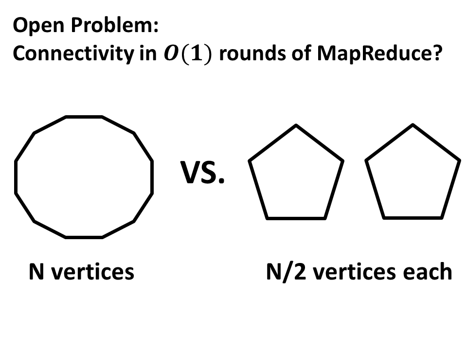
Open Problem
Is it possible to solve connectivity in constant number of rounds? This is a big open problem in the area and the consensus seems to be that this is not possible. In fact, it is open even whether one can distinguish a cycle on \(N\) vertices from two cycles on \(N/2\) vertices each in constant number of rounds.